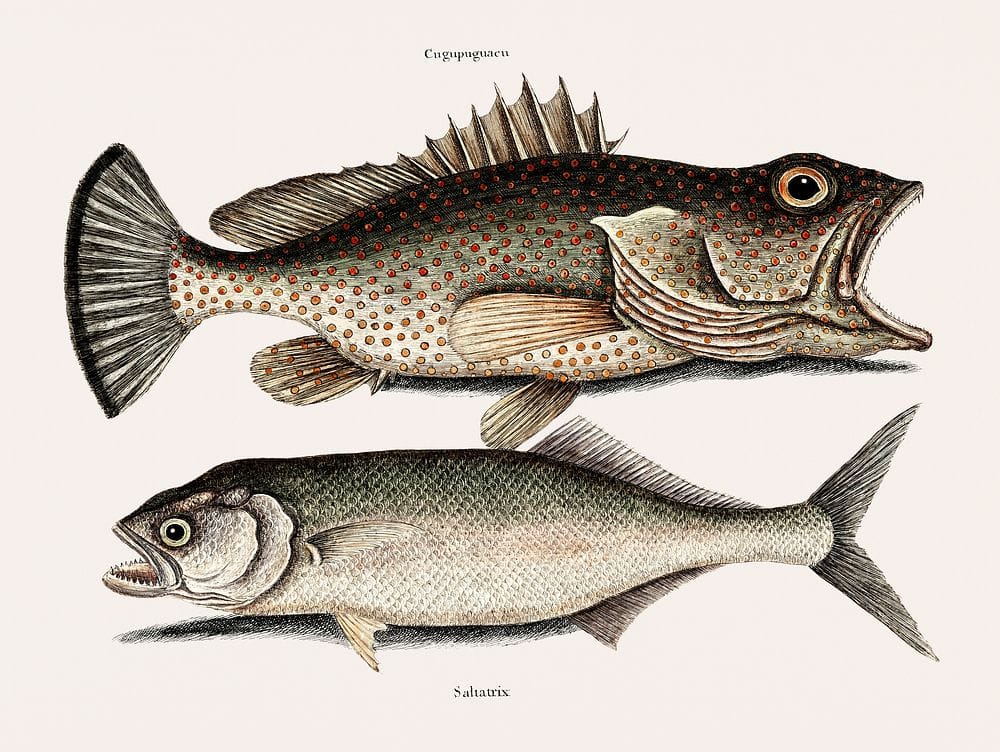
About fish and machine learning

This post intends to sum up and revise the contents of the first lecture in Machine Learning 1 at TU Berlin. The lecture uses an example and graphs from the book Pattern Classification by Duda et al. 2000.

Machine Learning is creating algorithms that can make predictions based on some (finite) data. The purpose of this is, that these machines can substitute or support human decision making, but also potentially serve to find underlying laws in the data.

The Bayes Decision Theory is a theoretical framework for building such decision models that yield optimal classifiers. It is theoretical in the sense that, in the real-world scenarios, the true underlying class probabilities and probability density functions are typically unknown.

Duda et al. introduce this decision model using the example of fish on a conveyor belt that is either salmon or sea bass. In machine learning, these objects of classification are referred to as "classes" and denoted with a vector \( \omega_1, \omega_2 ...\). To make a decision, Duda et al. describe a system collecting data through sensors, such as length or lightness. Other features, such as weight, could also be included. They refer to these parameters as a vector \( x \in \mathbb{R}^d\) , whose dimensions correspond to the number of parameters, defining the so-called feature space. For example, \( x_1\) could represent length and \( x_2\) could represent lightness.

Further, notation for probability laws is introduced:

\[ \mathbf{P (\omega_j)} \\ \text{ }\\ \text{"Probability that a fish belongs to class j"} \]

In this scenario, they consider only two types of fish and define their probabilities of appearing on the conveyor belt as\( P (\omega_1) \) (salmon) and \( P (\omega_2) \) (sea bass). Since these are the only two possibilities, these probabilities must sum to one. Depending on external factors, such as the season, one class of fish may be more likely than the other. If some prior knowledge about these probabilities is available, they are referred to as "prior probabilities."

\[ \mathbf{p(x|\omega_j)} \\ \text{ }\\ \text{"Density function of measurements x for each class j"} \]

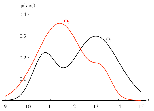
Now, it is not enough to make an accurate prediction of the next fish on the conveyor belt by just using the prior. The measurements \( x\) provide additional information for a more informed decision. The density function \( p(x|\omega_j) \) describes how likely it is that a fish of class j has the given measurements \( x\). This is why it is also referred to as the "likelihood."

\[ \mathbf{p(x) } \\ \text{ }\\ \text{"Density function of measurements x"} \]

This function describes the overall distribution of feature measurements for all fish. It is also called the 'evidence' because it represents the total probability of observing \( x\) across all classes.

Finally, the actual goal of the classifier is to determine: \[ \mathbf{P(\omega_j|x) } \\ \text{ }\\ \text{"The probability that a fish belongs to class j, given measurements x"} \]

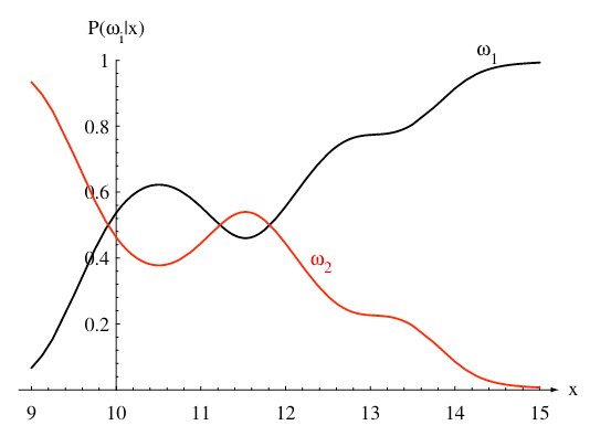
This is also referred to as the "posterior probability." These probability laws are connected through Bayes' Theorem:

\[ \mathbf{P (\omega_j | x) = \frac{p(x|\omega_j) \cdot P(\omega_j)}{p(x)}} \]

or

\[ \mathbf{posterior = \frac{likelihood \cdot prior}{evidence}} \]

To obtain an optimal decision function, we take the \[ \mathbf{ \text{arg max}_j P (\omega_j | x) = \text{arg max}_j \frac{p(x|\omega_j) \cdot P(\omega_j)}{p(x)}} \]

Since the denominator \(p(x)\) is independent of \(j\) , it does not affect the maximization and can be omitted. Next, we take the logarithm on both sides to transform the product into a sum. This is possible because the logarithm is a strictly increasing function, meaning it preserves the ordering of the arg max expression. This transformation simplifies calculations:

\[ \mathbf{ \text{arg max}_j \log P (\omega_j | x) = \text{arg max}_j \log p(x|\omega_j) + \log P(\omega_j)}\]

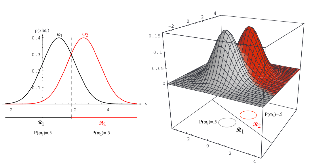
Now we assume that /( p(x|\omega_j) /) follows a multivariate normal distribution (also known as a Gaussian distribution):

\[ \mathbf{ p(x|\omega_j) = \frac{1} {\sqrt{(2\pi)^d \text{det}(\Sigma_j)} } } \text{exp}\left (-\frac{1}{2} (x-\mu_j) ^T \Sigma_j ^ {-1} (x-\mu_j) \right)\]

where \( \mu_j\) is the mean and \( \Sigma_j\) is the covariance matrix.

Substituting this into our optimal classifier, the fraction in the normal distribution can be ignored (since it does not depend on j), and the logarithm cancels out the exponentiation, leading to:

\[ \mathbf{ \text{arg max}_j \log P (\omega_j | x) = \text{arg max}_j \left (-\frac{1}{2} (x-\mu_j) ^T \Sigma_j ^ {-1} (x-\mu_j) \right) + \log P(\omega_j)}\]

Expanding the quadratic term, the first term is independent of j and can be omitted. The remaining terms can be rewritten in the familiar normal form of a hyperplane in \(\mathbb{R}^n\) respectively the linear decision boundary.

\[ \mathbf{ \text{arg max}_j \log P (\omega_j | x) = \text{arg max}_j - \cancel{\frac{1}{2} x ^T \Sigma_j ^ {-1} x} + \underbrace{x ^T \Sigma_j ^ {-1} \mu_j }_{ \vec w_j} - \underbrace{\frac{1}{2} \mu_j^T \Sigma_j ^ {-1} \mu_j + \log P(\omega_j)}_{ \vec b_j} }\]

\[ \mathbf{ \text{arg max}_j \log P (\omega_j | x) = \text{arg max}_j \, w_j ^T x + b_j }\]

This simplification holds when all covariance matrices \( \Sigma_j\) are equal; otherwise, the decision boundaries become quadratic instead of linear.

Sources:

• ML1 Lecture 1 , TU Berlin, WiSe 2024/25
• "Pattern Classification" by Duda et al. 2000