CCA is a method which finds projections \( w_x, w_y \) under which datapoints of 2 variables \(X,Y \) show maximal correlation, thus in a manner of speaking move in unison.

Let's start by giving the correlation we are seeking the greek letter \( \varrho \). Then we take scalar products of our data matrices \(X,Y \) with their respective projection vector, so we end up with 2 scalars:

\[ u = Xw_x , \quad v = Yw_y\]

Now, we use the standard definition of correlation as follows:

\[ \varrho = \mathrm{Corr}(u,v) = \frac{\mathrm{Cov}(u,v)}{\sqrt{\mathrm{Var}(u)}\sqrt{\mathrm{Var}(v)}}\]

when re-inserting our variables and their Co- and Autovariances \( C_{xy} = \frac{1}{N}XY^T, \quad C_{xx} = \frac{1}{N}XX^T, \quad C_{yy} = \frac{1}{N}YY^T \) we get:

\[ \varrho = \mathrm{Corr}(w_x,w_y) = \frac{w_x ^T C_{XY} w_y}{\sqrt{w_x ^T C_{XX} w_x} \sqrt{w_y ^T C_{YY} w_y}} \]

This above expression needs to be maximised in order to find the projections of highest correlation.

\[ \underset{w_x, w_y}{\mathrm{max}} \frac{w_x ^T C_{XY} w_y}{\sqrt{w_x ^T C_{XX} w_x} \sqrt{w_y ^T C_{YY} w_y}} \]

Maximisation mostly goes via derivation, hence the fraction is tedious to handle. Therefore we eliminate it by constraining the 2 Variances in the denominator to 1, which allows us to omit the denominator alltogether. So with \[w_x ^ T XX ^ T w_x = 1\] and \[ w_y ^ T YY ^ T w_y = 1\] we get \[ \underset{w_x, w_y}{\mathrm{argmax}} (w_x^T XY ^T w_y ) \] As a subtlety, you will have noticed that we went from above \( \underset{w_x, w_y}{\mathrm{max}} \) to \( \underset{w_x, w_y}{\mathrm{argmax}} \) . To make it clear, the first is maximising the actual resulting scalar, so the actual correlation value. The latter is more useful, as it's result is arguments \( w_x, w_y \) under which this maximum is found. Practically we will just care about these directions, less about the value of the correlation.

Now, some of you will already see that this can be solved with Lagrange. We have a maximisation problem and 2 constraints. Let's try to write this out. First, let's bring the constraints in the correct form:

\[w_x ^ T XX ^ T w_x -1 = 0 \] and \[w_y ^ T YY ^ T w_y -1 = 0 \]

\[ \underset{w_x, w_y}{L} = w_x^T C_{xy} w_y - \frac{1}{2}\alpha(w_x ^ T C_{xx} w_x -1) - \frac{1}{2}\beta(w_y ^ T C_{yy} w_y -1)\]

We add the \( \frac{1}{2} \) as it makes subsequent derivation of the squared variables \( w_x, w_y \) much easier. After derivation we set them to zero and bring one term over and multiply both sides.
\[ \begin{align*}\frac{\partial L}{\partial w_x^T } = C_{xy} w_y - \alpha C_{xx} w_x &= 0 \\ \alpha C_{xx} w_x &= C_{xy} w_y | \cdot w_x ^T \\ \alpha \underbrace{w_x ^T C_{xx} w_x}_{=1} &= w_x ^T C_{xy} w_y \end{align*} \]

\[ \begin{align*} \frac{\partial L}{\partial w_y^T } = C_{yx} w_x - \beta C_{yy}w_y &= 0 \\ \beta C_{yy} w_y &= C_{yx} w_x | \cdot w_y ^T \\ \beta \underbrace{w_y ^T C_{yy} w_y}_{=1} &= w_y ^T C_{yx} w_x \end{align*} \]

An additional note for the first term in the second derivation, as it can easily trip one up. \( (w_x^T C_{xy} w_y) ^T = w_y^T C_{xy} ^T w_x = w_y^T C_{yx} w_x \)

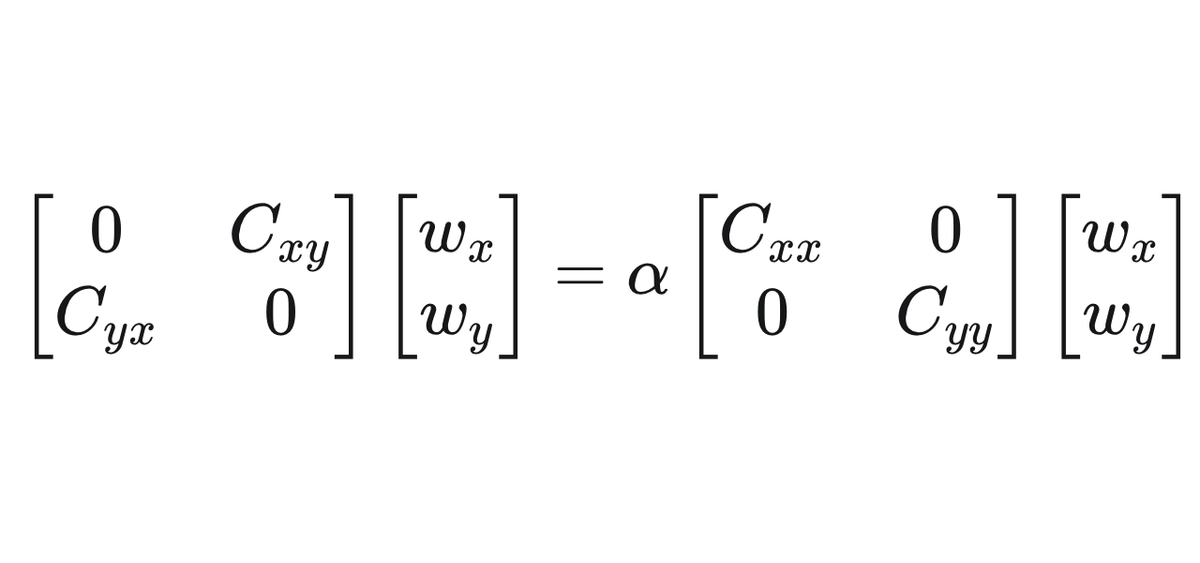
Most importantly we can see now that actually \( \alpha = \beta \) ! Our partial derivatives from above become: \[ \begin{align*} \alpha C_{xx} w_x &= C_{xy} w_y \\ \alpha C_{yy} w_y &= C_{yx} w_x \end{align*} \] Finally, we can write this in block matrix form which is a generalised eigenvalue equation:

\[ \begin{bmatrix} 0 & C_{xy} \\ C_{yx} & 0 \end{bmatrix} \begin{bmatrix} w_x \\ w_y \end{bmatrix} = \alpha \begin{bmatrix} C_{xx} & 0 \\ 0 & C_{yy} \end{bmatrix} \begin{bmatrix} w_x \\ w_y \end{bmatrix}\]

Arriving at this expression we can solve this using the standard solution for Eigenvalues / Eigenvectors : \[ Av = \lambda v \]

Much more can be done with CCA. For example, we can kernelize it to kCCA. This has the advantage of operating on the Kernels of the data and not on covariance matrices, which can become very large. Also, this allows us to model non-linear dependencies.