FDTD for Room Acoustics, Part 1: Deriving the 2D Wave Equation Solver

My long-term goal in this series is to build a small differentiable wave simulator for room-acoustics experiments. This first post starts with the simplest useful ingredient: a two-dimensional finite-difference solver for the homogeneous wave equation. The model is deliberately simplified, but it gives us the core update rule that later posts can extend with sources, boundaries, absorption, and eventually differentiability.

What is FDM?

The Finite Difference Method (FDM) provides a simple and powerful way to approximate partial differential equations. In this article, we derive an explicit finite-difference time-domain (FDTD) scheme for the two-dimensional wave equation, enabling us to simulate acoustic wave propagation in a medium.

The Wave Equation

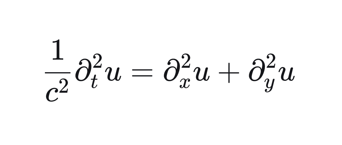
Let's start by writing down the homogeneous wave equation in 2D space and time for a variable \( u(x,y,t)\):
\[ u_{tt} = c^2 \left( u_{xx} + u_{yy} \right) \]
The subscripts indicate second order partial derivatives in time and space. The constant \( c\) denotes the wave propagation speed. In air at room temperature, this is usually approximated as \( 343 , \mathrm{ m/s} \).

We rearrange the equation to isolate the second derivative over time and the inverse of the squared wave propagation speed on the left side and the spatial second derivatives over \( x \) and \( y \) on the right side.

\[ \begin{split} \frac{1}{c ^2 } \partial ^2 _t u = \partial ^ 2 _x u + \partial ^2 _y u \end{split} \]

Discretisation and Approximation

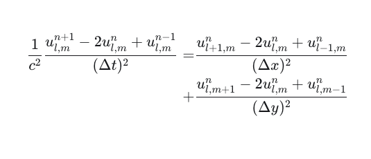
We now evaluate the PDE on a two-dimensional grid of points at discrete timesteps. Hence we define our discretized values \(u\) as follows. The indices \( l,m\) denote the steps in \(x\) and \(y\) directions, while \( n\) denotes the timestep:
\[ u ^n _{l,m} \approx u(l \Delta x, m \Delta y , n \Delta t)\]

Now we are replacing those derivatives with finite differences, which are a numerical approximation of the analytical derivatives. These finite-difference formulas can be derived by expanding neighbouring grid values in a Taylor series around the point of interest. As the wave equation contains second-order derivatives in time and space, we approximate them here with second-order central differences.

\[ \begin{split} \frac{1}{c^2} \frac{u ^{n+1} _{l,m} -2u ^{n} _{l,m} +u ^{n-1} _{l,m}}{ (\Delta t )^ 2} = &\frac{u ^{n} _{l+1,m} -2u ^{n} _{l,m} +u ^{n} _{l-1,m}}{( \Delta x) ^ 2} \\ + &\frac{u ^{n} _{l,m+1} -2u ^{n} _{l,m} +u ^{n} _{l,m-1}}{( \Delta y) ^ 2} \end{split}\]

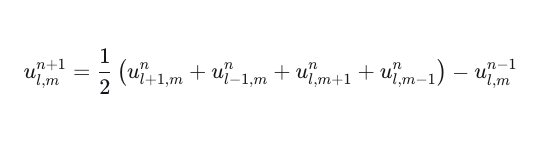
Then we refactor the equation so that we have the \( u^ {n+1}\) for the next timestep on the left and all space-dependent terms in groups on the right hand side. This gives us:

\[ \begin{split} u ^{n+1} _{l,m} = &2 u ^ {n} _{l,m} - u ^{n-1} _{l,m} + \\ &\frac{c ^2 \Delta t ^2}{ \Delta x ^2} \left ( u ^{n} _{l+1,m} - 2 u ^ {n} _{l,m} + u ^{n} _{l-1,m} \right ) + \\ &\frac{c ^2 \Delta t ^2}{ \Delta y ^2} \left ( u ^{n} _{l,m+1} - 2 u ^ {n} _{l,m} + u ^{n} _{l,m-1} \right ) \end{split} \tag{1}\]

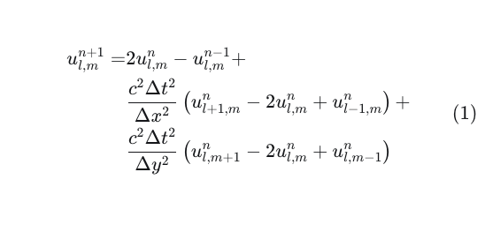
The update uses the value at \(u^n_{l,m}\) together with its four neighbouring grid points. This local pattern of points is often called a finite-difference stencil; in this case, it is a 5-point stencil. We will revisit this more concretely in the implementation in Part 2.

Ensuring stability of the scheme

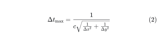
Now we include the Courant-Friedrichs-Lewy (CFL) condition for this 2 dimensional case. It is crucial for our scheme to remain stable.

\[ \frac{c ^2 \Delta t ^2}{ \Delta x ^2} + \frac{c ^2 \Delta t ^2}{ \Delta y ^2} \leq 1 \]

Rearranging this condition gives the maximum allowed timestep for the general case \( \Delta x \neq \Delta y \):

\[ \Delta t_{\max} = \frac{1}{c\sqrt{\frac{1}{\Delta x^2}+\frac{1}{\Delta y^2}}} \tag{2}\]

Now, assuming \( \Delta x = \Delta y \) we could further simplify the original expression to

\[ \begin{split} 2 \frac{c ^2 \Delta t ^2}{ \Delta x ^2} \leq 1 \ \end{split} \]
so
\[ \frac{c ^2 \Delta t ^2}{ \Delta x ^2} \leq \frac{1}{2} \]

If the CFL condition is saturated on a square grid with \( \Delta x = \Delta y \), then \( \frac{c ^2 \Delta t ^2}{ \Delta x ^2} = \frac{1}{2} \). When we insert this value into our update equation, we can see that the first term with the central node cancels. What remains is:

\[ u ^{n+1} _{l,m} = \frac{1}{2} \left ( u ^{n} _{l+1,m} + u ^{n} _{l-1,m} + u ^{n} _{l,m+1} + u ^{n} _{l,m-1} \right ) - u ^{n-1} _{l,m}\]

We can see that choosing the saturated CFL limit drastically simplifies the update. This special case is useful because it shows how the next value is built from neighbouring grid points and the previous time step. In the implementation, however, we will keep the more general form from equation (1), because it also works for rectangular grids and for timesteps below the CFL limit.

The CFL condition controls stability, but it does not remove the approximation error introduced by the grid. In particular, the propagation behaviour depends on the direction of travel: errors are more pronounced for axis-aligned waves than for diagonal ones. This behaviour is a manifestation of numerical anisotropy, a well-known property of finite-difference wave solvers. We will see this anisotropy in our tests once we have implemented the scheme in Part 2.

Dirichlet boundary condition

For a first implementation of this scheme, we also need to define boundary conditions for the two-dimensional domain. We will use a basic fixed boundary, where the field is set to zero on every boundary node. This is commonly referred to as a homogeneous Dirichlet boundary.

\[ u = 0 \quad \text{on } \partial \Omega. \]

When using this type of boundary we can observe a characteristic behaviour in the animation: after hitting the boundary, a red pressure maximum is reflected as a blue pressure minimum. In other words, the reflected wave changes sign. This is also called a phase inversion and is typical for this kind of boundary condition.

However, this boundary condition is closer to the behaviour of a fixed membrane than to the behaviour of typical room boundaries. For room acoustics, we will eventually need boundary models that better represent rigid walls, absorption, and impedance. This is something we will tackle in the next parts of the series.

Conclusion

We now have the ingredients for a first simulation: a discrete update rule (1), a stability condition for the timestep (2), and a simple boundary condition. In Part 2, we will translate the update rule directly into Python code using Dr.Jit, store the two-dimensional grid as a flattened array, and visualize the resulting wave propagation.

Sources and credits:

Brian Hamilton, "Tutorial on finite-difference time-domain (FDTD) methods for room acoustics simulation": https://www.youtube.com/watch?v=xgJJwmrX568
This tutorial was the main starting point for the FDTD derivation used in this post.

Numerics II for Engineers, TU Berlin, WS 2025/26 - Prof. Dr. Tobias Breiten, Prof. Dr. Sandra May, Dr. Juliette Dubois and Alireza Selahi Moghaddam,
This course provided much of the numerical-analysis background that helped me work through this material.