From Linear Regression to Polynomial Ridge Regression

This post is a recap of topics discussed in the 13th lecture of Machine Learning 1 at TU Berlin. Some of its aspects were also discussed in lecture 4 in the module Cognitive Algorithms at TU Berlin.

In contrast to classification which was discussed in lecture 1 of Machine Learning 1, Regression is commonly used for predicting real valued outputs. A practical example would be looking at prices (y-axis) of a commodity over time (x-Axis) and then drawing a curve through these points with as little deviation as possible.

Hypothesis function

For this basic example, we start by writing the equation for a line. From high school you might remember \( w \) being the steepness of a curve and \( b \) as the offset from the origin along the y-axis. The only difference with the following notation is that we can extend this concept to more dimensions:

\[ \hat y = w^Tx + b\]

To make things easier for subsequent calculations, we integrate the bias \( b \) into \( w \) as \( w_0 \). This only requires adding a \(1\) as \(x_0\) in our \(x\) array.

\[ \hat y = w^Tx + b = {\underbrace{[1,x]}_{x}}^T \underbrace{[b,w]}_{w} = w^Tx \]

Ordinary least squares (OLS) Error

Now, the question is how to fit the line to our datapoints. We need a measure for how poorly the fit performs. For that, we sum the deviations of each data point from our model’s predictions. Since we need positive-valued distances for the sum, we square the distances, which also has the effect of penalizing data points that are far away more heavily. We call this the Ordinary Least Squares Error (OLS):

\[ \text{Err}_{\text{OLS}} = \frac{1}{2}\sum_{i=1}^{n} ( w ^ T x_i - \hat y_i) ^ 2\]

Now, we need to find out which weights \(w\) yield the best result. Since the error is a convex function, we can set the first derivative of the error with respect to the weight \(w\) equal to zero to find the minimum. This also shows that the factor \(\frac{1}{2}\) cancels out the 2 resulting from the outer derivative, which is why it's often included:

\[ \begin{split}\frac{\partial \text{Err}_{\text{OLS}}}{\partial w} &= \frac{\partial }{\partial w} \frac{1}{2}\sum_{i=1}^{n} ( w ^ T x_i - \hat y_i) ^ 2\\&= \frac{\cancel{2}}{\cancel{2}} \sum_{i=1}^{n} ( w ^ T x_i - \hat y_i) x_i \\ &= 0 \end{split} \]

Switching to Matrix notation

Rewriting in matrix form requires careful attention to dimensions to avoid confusion:

\[ \begin{split}\frac{\partial \text{Err}{\text{OLS}}}{\partial w} &= \underbrace{ ( \underbrace{ \underbrace{ \underbrace{X}_{ n \times d} \underbrace{w }_{d \times 1} }_{n \times 1} - \underbrace{\hat y}_{n \times 1}) ^ T } _{1 \times n}\underbrace{X}_{ n \times d} }_{1 \times d \text{ (row vector)}} \\ &= \underbrace{X^T (Xw - \hat y) } _{d \times 1 \text{ (column vector)}} \\ &= 0 \end{split} \]

Actually, above definition of \( X \in \mathbb{R}^{n \times d}\) may seem a bit unusual, as we normally work with column vectors, so \( d\) should be the amount of rows not the amount of columns. In the literature you can see both and this might be confusing at times, so let's go through both versions here:

\[ \begin{split}\frac{\partial \text{Err}{\text{OLS}}}{\partial w} &= \underbrace{ ( \underbrace{ \underbrace{ \underbrace{w ^ T}_{d \times 1} \underbrace{X}_{ d \times n} }_{1 \times n} - \underbrace{\hat y}_{1 \times n}) } _{1 \times n}\underbrace{X ^ T}_{ n \times d} }_{1 \times d \text{ (row vector)}} \\ &= \underbrace{X (w ^ T X - \hat y) } _{d \times 1 \text{ (column vector)}} \\ &= 0 \end{split} \]

Closed solution for weights

We can solve now for \(w\) by reordering the equation for \( X \in \mathbb{R}^{n \times d}\) :

\[ \begin{split} X^T (Xw - \hat y) &= 0 \\ X^T Xw - X^T \hat y &= 0 \\ X^T Xw &= X^T \hat y \quad | \cdot (X^T X) ^ {-1} \\ w &= (X^T X) ^ {-1} X ^ T \hat y \end{split} \]

Respectively \(w\) for \( X \in \mathbb{R}^{ d \times n}\) :

\[ \begin{split} X (w ^ T X - \hat y) &= 0 \\ X w ^ T X - X \hat y &= 0 \\ X w^TX &= X \hat y \\ X X^Tw &= X \hat y \quad | \cdot (X X^T) ^ {-1} \\ w &= (X X^T) ^ {-1} X \hat y \end{split} \]

We have arrived at a closed-form solution for the hyperparameter \(w\). This allows us to compute \(w\) directly, making it a useful reference for understanding more advanced regression techniques.

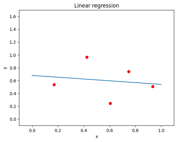
Let's now have a look at a simple linear regression example below. We can see that the line lies in between the sample points giving a rough match to an overall downward trend:

Polynomial regression (PR)

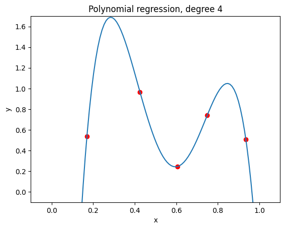
Our linear regression model fits the data to some extent, but it is limited to being a straight line. To capture more complex relationships, we can extend our model to polynomials. You might remember quadratic functions from high school, such as \(ax^2 + bx + c\). Generalizing to an nth-degree polynomial: \(w_nx^n + \dots w_2x^2 + w_1x + w_0\) By applying this transformation, we essentially map our original input to a higher-dimensional feature space, where a linear model can now fit curved patterns.

As you can see below, a 4th degree polynomial matches our sample data already perfectly.

PR Python Code

def polynomial_regression(x, y, degree):
    X = np.array([x**i for i in range(degree+1)]).T
    w = (np.linalg.pinv([email protected])@X).T@y[...,np.newaxis]
    return w

Overfitting

Now, the sample data has been matched perfectly, but let's take a step back. What if these data points contain noise? In that case, our model isn’t just capturing the underlying trend—it’s also fitting random fluctuations in the data. This means that while our function may match these exact points, it might perform poorly on new data. This phenomenon is called overfitting: the model learns the training data too well, at the cost of generalizing to unseen points.

Ridge regression

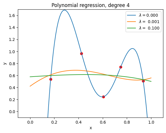
To combat overfitting, we introduce a penalty term that discourages large weights. This method is called Ridge Regression. By adding a regularization term, we trade some fit quality for better generalization. This approach introduces bias but reduces variance, improving the model’s ability to predict unseen data. The modified error function now includes a regularization term weighted by a hyperparameter \( \lambda \): \[ \text{Err}_{\text{OLS}} = \sum_{i=1}^{n} ( w ^ T x_i - \hat y_i) ^ 2 + \lambda \sum_{k=1}^{n} w_d ^ 2\] The larger we set \( \lambda \), the stronger the penalty on large coefficients, leading to a smoother model.

Polynomial Ridge Regression (PRR)

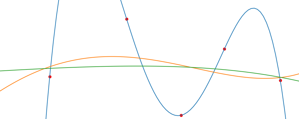
We can see that, depending on the choice of \( \lambda \), the sample points are more smoothly approximated, helping to avoid overfitting and thus better capturing the underlying trend in noisy data. In practice, this means we need to tune \( \lambda \) carefully to find the optimal balance between flexibility and regularization.

PRR Python Code

def polynomial_ridge_regression(x, y, degree, lmda):
    X = np.array([x**i for i in range(degree+1)]).T
    n = X.shape[0]
    w = (np.linalg.inv([email protected]+lmda*np.eye(n))@X).T@y[...,np.newaxis]
    return w

Final Thoughts

We’ve covered the progression from linear regression to polynomial regression and introduced ridge regularization to mitigate overfitting. In a follow-up post, we’ll explore how kernelized versions extend these ideas even further.