How a 19th Century Russian Mathematician Taught Us to Predict What Comes Next
Markov chains let us model sequences of events where each step depends only on the previous one. Learn how Andrey Markov’s 19th-century insight paved the way for modern applications in machine learning, finance, and beyond.
People have always been fascinated by predicting what comes next. If events are independent—like flipping a coin or rolling a die—prediction is straightforward. But in the real world, events are often interconnected: one event can influence another, which in turn affects the next, and so on. Trying to calculate probabilities across long chains of such events quickly becomes overwhelming.
Enter Andrey Markov, a 19th-century Russian mathematician. He discovered a clever simplification: to predict the next event in a sequence, you only need to know the immediately preceding event. This seemingly small insight made it possible to model complex systems of interconnected events—think weather patterns, stock prices, or even text generation—without needing impossible amounts of computation. Today, this idea forms the foundation of what we call Markov chains, a powerful tool for understanding and predicting sequences of events in an uncertain world.
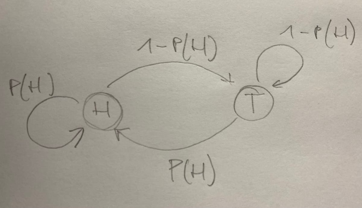
Now let's try to explain this a bit more in detail using an example. Let's start with the classic coin flip with heads and tails as outcomes. The diagram below illustrates these two States, Heads and Tails as well as the possible transitions in between. Naturally transitions can go from Heads to Tails and vice versa as well as can we remain in the same state (Heads - Heads, Tails - Tails) which is illustrated by the circular transitions.

Now we use this system and imagine flipping that coin a number of \( T \) times, resulting in \( q_1, \dots q_T \) timesteps, which take on our 2 state values Heads and Tails which we describe as \( \{S_1 , S_2\}\). For systems which have more than 2 state variables we can write more generally \( \{S_1, \dots , S_N\}\), so \( q_t \in \{S_1, \dots , S_N\}.\) To be precise, we refer here to \( q \) as timesteps, but as they take on the value of a state they are actually random variables. As for the arrow in between our two states above, they are directional as well as having a certain probability. As Probabilities need to sum to one, we have a Probability for Heads \( P(H) \) and \( 1 - P(H) \) for Tails. Let's say the coin is biased showing Heads more often than Tails, then the probabilities are something like \( P(H) = 0.6 \) and \( 1 - P(H) = 0.4 \).
Now, we would like to describe the probabilities after a certain amount of timesteps. As the Markov model can be seen as a joint distribution of the random variables / timesteps these probabilities. The key here is that each probability is always dependent on the previous step. Thus it can be described as follows: \[ P(q_1,\dots ,q_T) = P(q_1) \cdot \prod_{t= 2}^T P(q_t | q_{t-1}) \] Let's write it out until \( T\) without the product sign: \[ P(q_1 ,q_2, \dots ,q_T) = P(q_1) P(q_2 | q_{1}) \cdot \dots \cdot P(q_t | q_{t-1}) \], and to make it even more clear let's write as short 3 timestep chain: \[ P(q_1 ,q_2, q_3) = P(q_1) P(q_2 | q_{1}) P(q_3 | q_{2}) \]
Now our question will probably be, how do we calculate a probability at a certain timestep \( q_t \) with a certain state \( S_j \) , so \( P(q_t = S_j) = \) ?. To solve this we need to be aware that there is actually multiple ways of arriving at a certain state after a certain amount of timesteps. Let's say our initial state is Heads and we want to be again at Heads after 2 steps. Then we could either go Heads - Tails - Heads or Heads - Heads - Heads. This means we need to sum for every timestep those probabilities to represent all possible paths leading to \( S_j \), a process known as marginalisation, where we sum over the previous timesteps’ states because we only care about the probability of the current state. Let's try this for 3 timesteps using the joint Probability from above. What we need to define first is some abbreviations, otherwise even for a simple example, this becomes a very long expression. So let's denote the initial states with \( \pi_i = P(q_1 = S_i) \) and the transition probabilities with \( a_{ik} = P(q_{t+1} = S_k \mid q_t = S_i )\).
\[ \begin{split} P(q_3 = S_j) &= \sum_{q_1}\sum_{q_2} P(q_1 ,q_2, q_3 = S_j) \\ &= \sum_{q_1 \in \{S_1, S_2\}}\sum_{q_2 \in \{S_1, S_2\}} P(q_1), P(q_2 \mid q_{1})\, P(q_3 = S_j \mid q_{2}) \\ &= \pi_{1} a_{11}a_{1j} +\pi_{1} a_{12}a_{2j} + \pi_{2} a_{21}a_{1j}+ \pi_{2} a_{22}a_{2j}\\ \end{split} \] Now we can group expressions further: \[ \begin{split} P(q_3 = S_j) &= (\pi_{1} a_{11} + \pi_{2} a_{21}) a_{1j} + (\pi_{1} a_{12} + \pi_{2} a_{22}) a_{2j} \end{split}\] And the terms in the brackets are actually: \[ P(q_2 = S_1) = (\pi_{1} a_{11} + \pi_{2} a_{21}) , \quad P(q_2 = S_2) =(\pi_{1} a_{12} + \pi_{2} a_{22}) \] So this can be further compacted as follows: \[ P(q_3 = S_j) = \sum_{i=1}^N \left ( \sum_{r=1}^N \pi_{r} a_{ri} \right ) a_{ij} = \sum_{i=1}^{2} P(q_2 = S_i ) a_{ij} \]
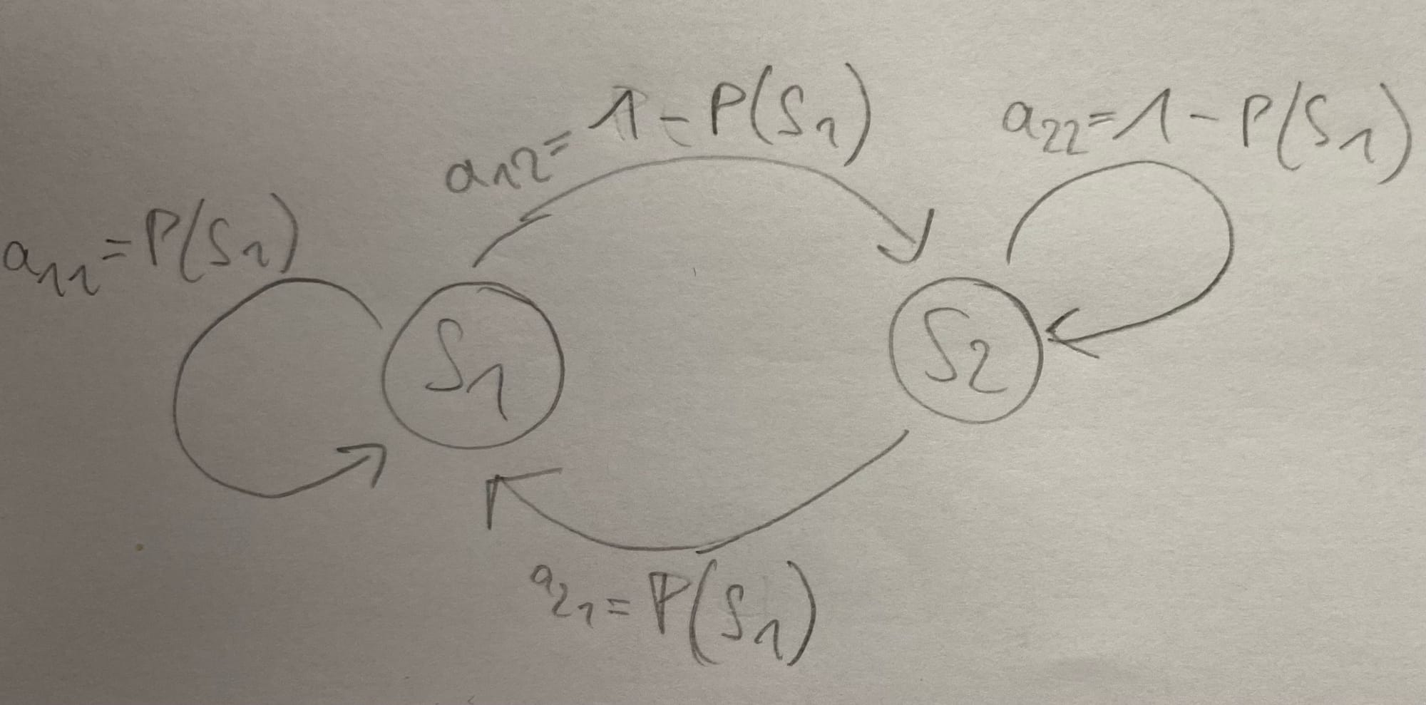
Now let's try to calculate this with the previously mentioned probabilities of a biased coin. For that purpose let's update our little diagram to match above variables:
Now we can individually write out that sum of products, but there is a better way by setting up an initial state vector \(\pi = \begin{bmatrix} 0.6 \\ 0.4 \end{bmatrix} \) and the transition matrix \(A = \begin{bmatrix} 0.6 & 0.4 \\ 0.6 & 0.4 \end{bmatrix} \). Now for 3 timesteps we can update our state vector as follows: \[ \pi^{(3)} = \pi A^2 \]. Let's calculate this quickly by hand and look at the result below:
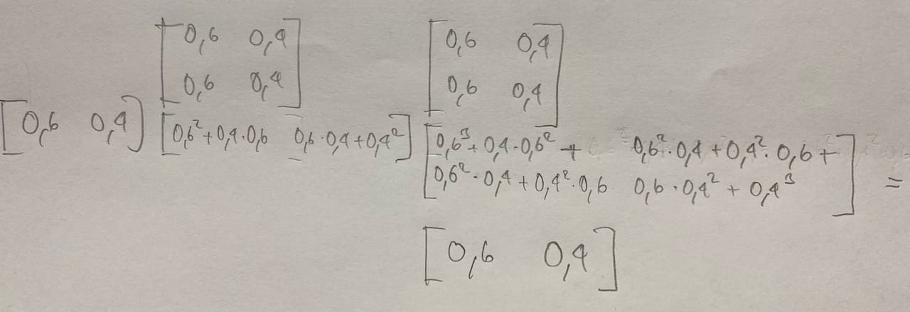
Ok, this is rather boring, isn't it ? Same result as the input. What happened ? Well, our coin example above is actually a perfect example for independent events, as normally the probabilities for Heads and Tails stay the same for every toss. So our math is correct, but the Markov chain cannot shine here, as the probabilities in the rows of the transition Matrix keep staying the same for every time step.
So let's change this example to a case where probabilities will change depending in which state we have been before. The simplest update to our hypothetical scenario with the coin would be, that we introduce a belief that after we tossed Head it is more likely to stay with Head then going to Tails next. We could express this as follows: \[A = \begin{bmatrix} 0.8 & 0.2 \\ 0.6 & 0.4 \end{bmatrix} \]
import numpy as np
A = np.array([[0.8, 0.2],[0.6, 0.4]])
pi = np.array([0.6, 0.4])
pi = pi @ A @ A
The result for the update is \(\pi^{(3)} = \pi A^2 = \begin{bmatrix} 0.744 \\ 0.256 \end{bmatrix} \) which shows that our belief now gets accounted for and the coin toss is dependent on previous results. If we repeat this calculation many times, the state distribution will converge to a stationary distribution, meaning, that it becomes a general distribution of results.
Markov chains are so useful because they propagate probabilities step by step, making complex systems more tractable. They have found applications in areas ranging from speech recognition and stock market prediction to natural language processing. Interestingly, they can even be seen as conceptual ancestors of the Attention mechanism, which underpins the power of today’s Large Language Models.
There is much more to say about Markov chains—maybe in a future post. Until then.
Sources: