Running LLMs on Your Own Hardware: A First Look
A first look at why people run LLMs locally, what hardware matters most, and why real-world performance is more complicated than the spec sheet suggests.
Introduction
Large Language Models (LLMs) have become a versatile tool in many people's workflows. Programmers use them to write code, in education they support teaching and learning, in research they help analyse data and generate ideas and companies are rapidly adopting them to automate parts of their businesses.
Many people, myself included, begin this journey with browser based tools like OpenAI's ChatGPT, DeepSeek or Anthropic's Claude. Free plans or mid-tier subscriptions already allow a substantial amount of work to be done, and for the most part they provide access to some of the best models currently available.
If these tools from large providers are both affordable and high quality, why would anyone look for other ways of accessing LLMs?
Why go Local ?
In fact, there are several reasons why many people choose to run LLMs on their own hardware. The most important one is privacy. With every prompt, data is sent to and processed in the data centres of the respective provider and is often stored there for some time. This is not only a concern for individuals, but especially for companies that need to ensure sensitive data is not exposed to third parties. The issue has become even more relevant in light of rising geopolitical tensions and growing scepticism toward large private corporations monetising user data, including by using it to train future models.
Another strong reason, somewhat surprisingly, is end-user cost. Some larger companies that rely heavily on LLMs are beginning to realise that the compute cost of using them for writing and maintaining large codebases can become substantial. This problem may become more pronounced in the future, as many major providers currently operate at a loss in order to gain market share. Given the enormous cost of building and running large data centres, today’s prices may not reflect the true long-term cost of these services.
Finally, the local path offers a much wider choice of models from platforms such as Hugging Face, rather than a small number of proprietary models that providers can change or remove at any time. Some of these models are truly open source, which means they can even be retrained for specific tasks and adapted more closely to a particular use case.
Is going Local the solution ?
Running a local LLM means running freely available models on your own hardware. In terms of privacy, this is hard to beat: your data stays on your own machine and remains under your control. Apart from electricity, the running cost is relatively low and the model is always available. The major cost factor is the hardware itself, especially the Graphics Processing Unit (GPU), which can be expensive depending on your requirements. However, hardware suitable for LLMs tends to retain its value relatively well because demand remains high and availability is often limited. Setting up a local LLM is surprisingly straightforward and generally well documented, although the exact process depends on the hardware being used.
Why is then not everyone doing this ?
One limitation is the relationship between hardware cost and the quality of the models you can run on it. For LLMs, it is roughly true that larger models tend to produce better results. The models used by OpenAI or Anthropic are extremely large and would not fit into the GPU memory of typical consumer hardware. In practice, such models are run across server-grade GPUs costing many tens of thousands of dollars.
However, smaller and more specialised models can still perform very well in a carefully balanced local setup, especially when adapted to a specific use case. This also means that finding the right setup takes time and experimentation. Compared with a commercial provider, the local route is less plug-and-play. On the other hand, anyone willing to go down that path will also gain valuable insight into how these systems actually work.
Which hardware is good for a local LLM ?
As mentioned above, the most important piece of hardware for running a local LLM is the GPU. Its chip is optimised for the parallel processing of large matrices using thousands of relatively simple cores. This makes it much faster for this kind of workload than a Central Processing Unit (CPU), which typically has far fewer cores and is better suited to more complex, general-purpose tasks.
For a long time, this market has been dominated by NVIDIA. This is not only because the company produces very capable hardware, but also because it provides a mature software framework that makes this computing power accessible beyond graphics processing. That framework is called CUDA. In recent years, NVIDIA’s main competitor AMD has been catching up with its own software stack, ROCm. Judging from AMD’s recent partnerships with companies such as OpenAI and Anthropic, it seems clear that both its chips and software have improved enough to make it an increasingly viable option.
There are also more specialised alternatives, such as Tensor Processing Units (TPUs), although these are often not available on the consumer market.
Finally, there is one more rather unlikely player in this space: Apple. Although better known for sleek laptops, phones, and tightly integrated services, Apple has become relevant here as a side effect of replacing Intel chips in its Mac lineup with its own ARM-based processors. Apple had already spent years designing efficient chips for iPhones and iPads, and in 2020 it introduced the M-series processors for Macs. This transition had a significant impact. Not only were these chips highly efficient and powerful, but they also introduced an architecture in which system memory is shared dynamically between CPU and GPU. While shared memory is not a new idea in itself, Apple’s implementation offers unusually high memory bandwidth. As we will see shortly, this is one of the key factors influencing how quickly an LLM can process and answer prompts. For example, the M1 Pro, M1 Max, and M1 Ultra offer memory bandwidths of 200, 400, and 800 GB/s respectively — values usually associated with dedicated GPUs from NVIDIA or AMD.
What about that bandwidth?
Before talking about bandwidth, we should establish one key concept: prompting an LLM is commonly referred to as inference. This is opposed to training an LLM, which is usually only done by large labs and requires thousands of hours of computation in data centres. In this article, we will focus on inference only.
LLM inference consists of two stages: prefill (prompt processing) and decode (token generation). Prefill processes the input prompt and constructs the KV-cache, while decode generates output tokens sequentially using this cache. In this article, token throughput measurements refer to decode performance unless otherwise stated.
Hardware memory bandwidth is especially relevant for the decode stage, which strongly influences the user experience. We usually describe how quickly an LLM generates text in tokens/s . Tokens are not exactly words, but rather words, fragments of words, or punctuation marks.
Average reading speed is roughly 200–250 words per minute. If one word corresponds to about 1.7 tokens on average, this results in approximately 5.6–7.1 tokens/s. A model generating text much more slowly than that may feel sluggish in interactive use.
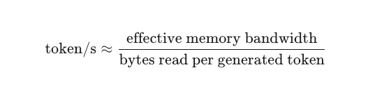
We can now define a simple theoretical upper bound for token generation that assumes a bandwidth-limited process.
A practical example
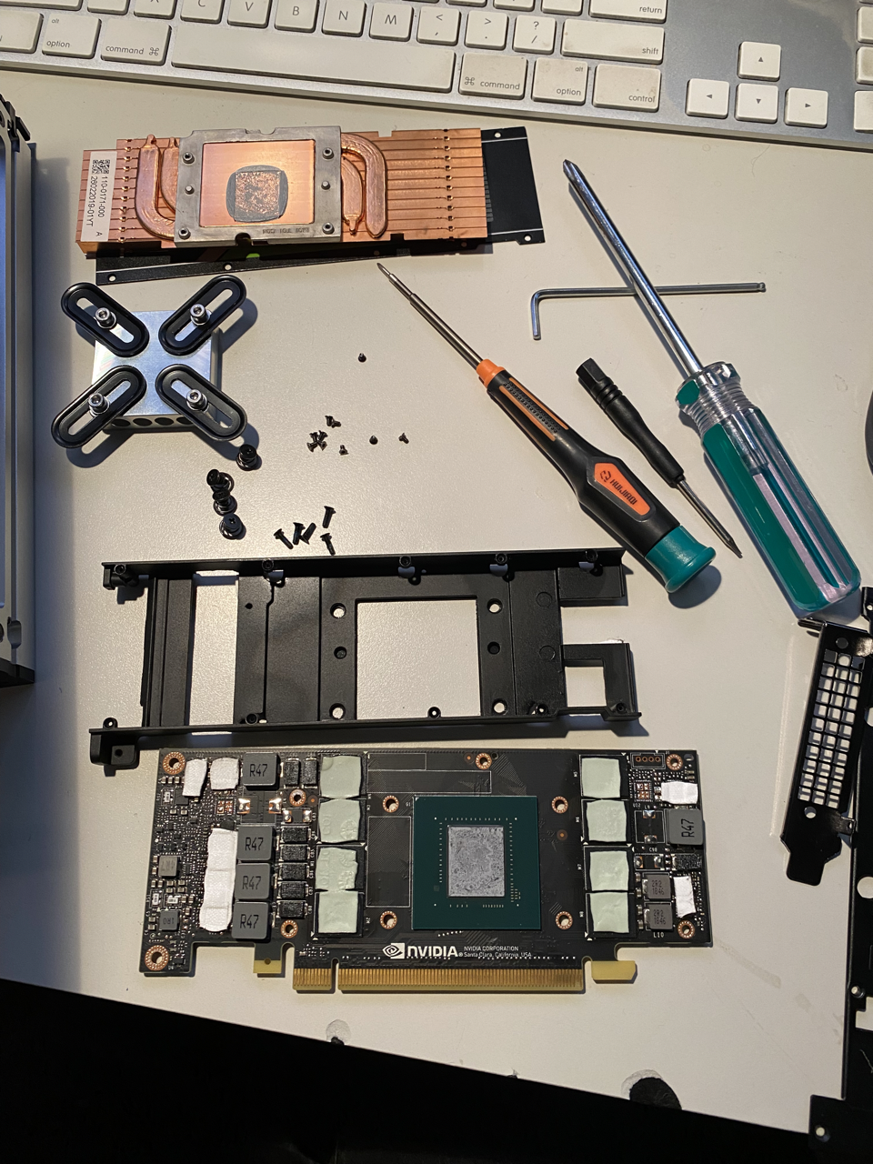
Let us now look at a simple example using a piece of hardware I own myself: an NVIDIA Tesla P4. This is an older card from 2016, designed primarily for inference and for continuous use in a server environment.
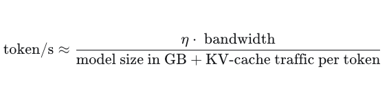
The Tesla P4 has 8 GB of VRAM, a memory bandwidth of 192.3 GB/s, and a maximum power draw of 75 W. To approximate real inference behavior, we model token generation as a bandwidth-limited process that accounts for both model weights and KV-cache traffic.
where
- \( \eta \) is a lumped implementation factor that captures all deviations from the idealized bandwidth model, including software, hardware, and model-dependent inefficiencies.
model sizebeing the actual size of the model weights in GPU memoryKV-cachedescribes the size of your context window. A context window is the maximum length of a conversation you can have with your LLM. In a local LLM you can set this length manually, but most models have a maximum length restriction. Especially for long coding or conversation sessions, this is a crucial parameter in terms of perceived quality of a LLM. The KV-cache is empty at the start and grows with each processed token. Therefore, inference speed depends on the current cache size rather than the maximum context window. As this value is in the denominator of our formula, you can see that token generation should become slower the longer the conversation goes on.
To estimate how fast an LLM will run on the Tesla P4, we first need to choose a suitable model. It must fit entirely into the card’s 8 GB of VRAM while still leaving some space for the context window and a small amount of overhead. If part of the model has to be stored in system memory instead, generation becomes much slower because regular RAM has far lower bandwidth than VRAM. In that case, the simple approximation above is no longer sufficient, since one would need to account for two different memory systems and the data transfer between them.
Given the VRAM limits of the Tesla P4, I chose Google’s recent Gemma Edge model in a 4-bit quantised version from Hugging Face, which has a size of 2633.88 MiB. This model runs in a forked version of llama.cpp . At the maximum context window size of 131,000 tokens, the KV-cache occupies 2048.00 MiB. Model overhead and KV-cache overhead account for roughly another 1 GB, so in total the setup uses about 5640 MiB of the 7680 MiB effectively available on the card.
Plugging these numbers into the theoretical memory bandwidth-bound upper limit gives:

This would be an excellent speed in theory — faster than most people can comfortably read.
However, this value assumes a fully filled context window. At low KV-cache occupancy (e.g. at the start of a conversation), KV-cache traffic is minimal, yielding an even higher theoretical upper bound:
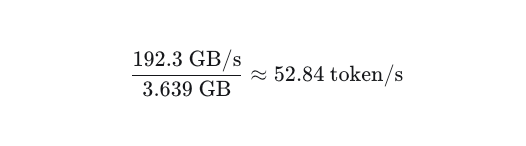
In practice, opening a fresh chat in the llama.cpp web interface with this model results in only about 9.79 tokens/s. It therefore makes sense to introduce the lumped implementation factor, η, into the formula:

This means that, for the hardware and software used in this experiment, the system reaches roughly 19% of the idealized memory-bandwidth limit. While the estimate is crude, it shows that memory bandwidth alone is not sufficient to predict real-world inference performance.
| Run P4 | Context at start | KV-cache size (MiB) | Eval time (ms) | Tokens/s | Eta |
|---|---|---|---|---|---|
| 1 | 30 | 5.28 | 62933.70 | 9.79 | 0.185 |
| 2 | 417 | 12.90 | 84755.39 | 9.64 | 0.183 |
| 3 | 1233 | 22.07 | 78598.06 | 9.55 | 0.181 |
From the table above, we can see that token generation speed does indeed depend on context length, slowing slightly as more data accumulates in the KV cache. At the same time, \( \eta \) remains in a fairly narrow range, although it becomes marginally lower. This again suggests that the simplified formula captures a useful part of the relationship, even if it does not describe all of the underlying behaviour.
As a comparison, I also ran the same model on the NVIDIA Tesla T4, the 2018 successor to the P4. It has a slightly lower 70 W power limit, includes tensor cores and offers 320.0 GB/s - about 66% more memory bandwidth than the P4 . In a first test, generation speed increased by only about 15% to 11.1 tokens/s , which was an unexpectedly small improvement.
Using the same back-of-the-envelope estimates, we get:
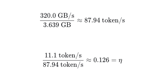
The empirical lumped implementation factor is therefore even lower here than on the P4. This does not mean that the T4 is inherently worse. Rather, it shows once again that real-world inference performance depends on more than raw memory bandwidth alone. In fact, after some troubleshooting, it turned out that the Docker container had been compiled for an older CUDA architecture compatible with the P4 . Rebuilding it for a more recent CUDA target changed the picture completely. On an identical first prompt, the T4 generated at 36.42 tokens/s , more than three times the previous speed. With a newer generation of hardware and a better-matched software stack, we therefore also obtain the higher \( \eta \) we expect:
\[ \frac{36.42\text{ token/s} }{87.94 \text{ token/s}} \approx 0.414 = \eta\]
| Run T4 | Context at start | KV-cache size (MiB) | Eval time (ms) | Tokens/s | ETA |
|---|---|---|---|---|---|
| 1 | 30 | 4.29 | 13426.70 | 36.42 | 0.414 |
| 2 | 398 | 12.44 | 22101.69 | 36.06 | 0.410 |
| 3 | 1194 | 20.66 | 24995.56 | 35.85 | 0.408 |
Across several runs, the T4 shows the same general pattern as the P4: generation speed decreases slightly as the context grows, while \( \eta \) remains within a fairly narrow range. The difference is that this happens at a much higher overall performance level.
Conclusions
The main takeaway is that local LLM performance cannot be reduced to a single number from a specification sheet. Memory bandwidth is clearly important, but real-world inference speed also depends on the software stack and on the length of the active context. The examples above are therefore best understood not as a complete benchmark, but as a practical attempt to make these relationships visible.